Assemblage
The Assemblage represents all of the things that can potentially be discovered within an Area. These are most commonly going to be artifacts represented as points, but can theoretically be other shapes as well. The Assemblage must lie within the Area, so an Area object is a required parameter of the Assemblage creation methods.
An Assemblage is made from a list of Layer objects, so most of the heavy lifting is done by creating each Layer. We will walk through Layer creation methods first, then we will put them together in an Assemblage.
Creating a Layer
A Layer is intended to be a group of artifacts or other features that share time_penalty and ideal_obs_rate parameters. More practically, you can think of a Layer standing in for a type of artifact. For example, you might expect those parameters to be the same for any Iron Age ceramics, so you can put all of the Iron Age ceramics into the same Layer.
Each element of the Layer (i.e., each individual artifact) is a Feature object. Most of the time it will make more sense to use Layer methods to create many Feature objects at the same time, but it is possible to create the Feature objects one-by-one and assembling them into a Layer.
From a list of Feature objects
To create a Feature, we need a shapely object, so let’s create a few simple points.
from shapely.geometry import Point
import prospect
from scipy.stats import beta

pt1 = Point(10, 10)
ft1 = prospect.Feature(
    name="feature1",
    layer_name="demo_layer",
    shape=pt1,
    time_penalty=prospect.utils.truncnorm(mean=10, sd=7, lower=0, upper=50),
    ideal_obs_rate=beta(9, 1)
)

pt2 = Point(50, 50)
ft2 = prospect.Feature(
    name="feature2",
    layer_name="demo_layer",
    shape=pt2,
    time_penalty=prospect.utils.truncnorm(mean=10, sd=7, lower=0, upper=50),
    ideal_obs_rate=beta(9, 1)
)

pt3 = Point(90, 90)
ft3 = prospect.Feature(
    name="feature3",
    layer_name="demo_layer",
    shape=pt3,
    time_penalty=prospect.utils.truncnorm(mean=10, sd=7, lower=0, upper=50),
    ideal_obs_rate=beta(9, 1)
)
Note
Notice that we kept the time_penalty and ideal_obs_rate parameters constant. It is not required that all members of a Layer have identical values for these parameters, but it is probably a good idea. If you need to use different values, it is probably best to use one Layer per unique set of parameters.
Now let’s put our Feature objects into a Layer. The Layer constructor will check and ensure that the Feature objects are located within the Area boundaries, so you must pass an Area when creating a Layer.
Note
Currently this spatial rule is only enforced if all of the elements in input_features are Point objects. It is my hope to include LineString and Polygon Feature objects in this “clipping” operation in the future.
demo_area = prospect.Area.from_area_value(
    name='demo_area',
    value=10000
)
layer_from_list = prospect.Layer(
    name='demo_layer',
    area=demo_area,
    input_features=[ft1, ft2, ft3]
)
type(layer_from_list)
prospect.layer.Layer
layer_from_list.df
| feature_name | layer_name | shape | time_penalty | ideal_obs_rate | |
|---|---|---|---|---|---|
| 0 | feature1 | demo_layer | POINT (10.00000 10.00000) | <scipy.stats._distn_infrastructure.rv_frozen o... | <scipy.stats._distn_infrastructure.rv_frozen o... |
| 1 | feature2 | demo_layer | POINT (50.00000 50.00000) | <scipy.stats._distn_infrastructure.rv_frozen o... | <scipy.stats._distn_infrastructure.rv_frozen o... |
| 2 | feature3 | demo_layer | POINT (90.00000 90.00000) | <scipy.stats._distn_infrastructure.rv_frozen o... | <scipy.stats._distn_infrastructure.rv_frozen o... |
type(layer_from_list.df)
geopandas.geodataframe.GeoDataFrame
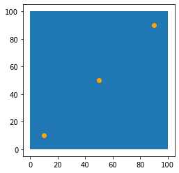
We can use the plotting functionality from geopandas to visualize the Layer members within the Area.
layer_from_list.df.plot(ax=demo_area.df.plot(), color="orange")
<AxesSubplot:>
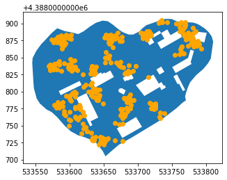
From a shapefile
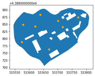
The from_shapefile() method is useful for reading in existing datasets as Layer objects. These could be data from a completed field survey or maybe data designed to test some custom question.
area_from_shp = prospect.Area.from_shapefile(
    name="area_shp",
    path="./data/demo_area.shp"
)

layer_from_shp = prospect.Layer.from_shapefile(
    path="./data/demo_layer.shp",
    name="demo_layer_from_shp",
    area=area_from_shp,
    time_penalty=prospect.utils.truncnorm(mean=10, sd=7, lower=0, upper=50),
    ideal_obs_rate=beta(9, 1)
)
layer_from_shp.df
| feature_name | layer_name | shape | time_penalty | ideal_obs_rate | |
|---|---|---|---|---|---|
| 0 | demo_layer_from_shp_0 | demo_layer_from_shp | POINT (533579.123 4388848.757) | <scipy.stats._distn_infrastructure.rv_frozen o... | <scipy.stats._distn_infrastructure.rv_frozen o... |
| 1 | demo_layer_from_shp_1 | demo_layer_from_shp | POINT (533638.844 4388883.594) | <scipy.stats._distn_infrastructure.rv_frozen o... | <scipy.stats._distn_infrastructure.rv_frozen o... |
| 2 | demo_layer_from_shp_2 | demo_layer_from_shp | POINT (533621.702 4388842.121) | <scipy.stats._distn_infrastructure.rv_frozen o... | <scipy.stats._distn_infrastructure.rv_frozen o... |
| 3 | demo_layer_from_shp_3 | demo_layer_from_shp | POINT (533701.882 4388861.475) | <scipy.stats._distn_infrastructure.rv_frozen o... | <scipy.stats._distn_infrastructure.rv_frozen o... |
| 4 | demo_layer_from_shp_4 | demo_layer_from_shp | POINT (533669.810 4388763.047) | <scipy.stats._distn_infrastructure.rv_frozen o... | <scipy.stats._distn_infrastructure.rv_frozen o... |
| 5 | demo_layer_from_shp_5 | demo_layer_from_shp | POINT (533575.252 4388787.930) | <scipy.stats._distn_infrastructure.rv_frozen o... | <scipy.stats._distn_infrastructure.rv_frozen o... |
| 6 | demo_layer_from_shp_6 | demo_layer_from_shp | POINT (533771.556 4388874.194) | <scipy.stats._distn_infrastructure.rv_frozen o... | <scipy.stats._distn_infrastructure.rv_frozen o... |
| 7 | demo_layer_from_shp_7 | demo_layer_from_shp | POINT (533717.918 4388839.910) | <scipy.stats._distn_infrastructure.rv_frozen o... | <scipy.stats._distn_infrastructure.rv_frozen o... |
Let’s plot the resulting Layer.
layer_from_shp.df.plot(ax=area_from_shp.df.plot(), color="orange")
<AxesSubplot:>
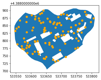
From pseudorandom points
To very quickly create a Layer with a specific number of points, you can use the from_pseudorandom_points() method. This method uses numpy to draw \(n\) random values for coordinates for Point objects.
area_from_shp = prospect.Area.from_shapefile(
    name="area_shp",
    path="./data/demo_area.shp"
)

layer_from_pseudo_rand = prospect.Layer.from_pseudorandom_points(
    n=100,
    name="demo_layer_from_pseu_rand",
    area=area_from_shp,
    time_penalty=prospect.utils.truncnorm(mean=10, sd=7, lower=0, upper=50),
    ideal_obs_rate=beta(9, 1)
)
layer_from_pseudo_rand.df.shape
(100, 5)
layer_from_pseudo_rand.df.plot(ax=area_from_shp.df.plot(), color='orange')
<AxesSubplot:>
From point processes
prospect offers methods for creating Layer objects using existing point pattern types: Poisson, Thomas, and Matern.
Caution
For all of these point pattern types, the generated points are not guaranteed to fall within the given Area, only within its bounding box. The generated GeoDataFrame of points, df, is clipped by the actual Area bounds after they are generated, which can result in fewer points than expected. If you need to examine what has been clipped, all original points will remain in the input_features attribute.
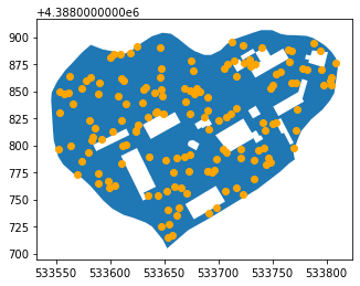
Poisson
A Poisson point process is usually said to be more “purely” random than most random number generators (like the one used in from_pseudorandom_points())
The rate (usually called “lambda”) of the Poisson point process represents the number of events per unit of area per unit of time across some theoretical space of which our Area is some subset. In this case, we only have one unit of time, so the rate really represents a theoretical number of events per unit area. For example, if the specified rate is 5, in any 1x1 square, the number of points observed will be drawn randomly from a Poisson distribution with a shape parameter of 5. In practical terms, this means that over many 1x1 areas (or many observations of the same area), the mean number of points observed in that area will approximate 5.
area_from_shp = prospect.Area.from_shapefile(
    name="area_shp",
    path="./data/demo_area.shp"
)

layer_from_poisson = prospect.Layer.from_poisson_points(
    rate=0.005,
    name="demo_layer_from_poisson",
    area=area_from_shp,
    time_penalty=prospect.utils.truncnorm(mean=10, sd=7, lower=0, upper=50),
    ideal_obs_rate=beta(9, 1)
)
layer_from_poisson.df.shape
(151, 5)
layer_from_poisson.df.plot(ax=area_from_shp.df.plot(), color='orange')
<AxesSubplot:>
Thomas
A Thomas point process is a two-stage Poisson process. It has a Poisson number of clusters, each with a Poisson number of points distributed with an isotropic Gaussian distribution of a given variance. The points that are used to define the parent clusters are not represented in the output.
Tip
This is an excellent way to generate artifact clusters.
area_from_shp = prospect.Area.from_shapefile(
    name="area_shp",
    path="./data/demo_area.shp"
)

layer_from_thomas = prospect.Layer.from_thomas_points(
    parent_rate=0.001,
    child_rate=10,
    gauss_var=5,
    name="demo_layer_from_thomas",
    area=area_from_shp,
    time_penalty=prospect.utils.truncnorm(mean=10, sd=7, lower=0, upper=50),
    ideal_obs_rate=beta(9, 1)
)
layer_from_thomas.df.shape
(324, 5)
layer_from_thomas.df.plot(ax=area_from_shp.df.plot(), color='orange')
<AxesSubplot:>
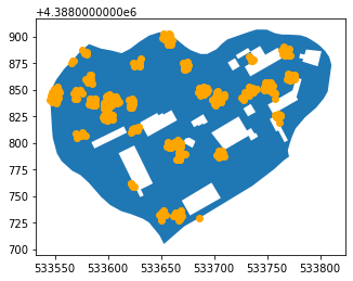
Matern
The Matern process is similar to the Thomas point process. It has a Poisson number of parent clusters like the Thomas process, but in this case, each parent cluster has a Poisson number of points distributed uniformly across a disk of a given radius.
Tip
This is an excellent method for generating circular clusters of artifacts.
area_from_shp = prospect.Area.from_shapefile(
    name="area_shp",
    path="./data/demo_area.shp"
)

layer_from_matern = prospect.Layer.from_matern_points(
    parent_rate=0.001,
    child_rate=10,
    radius=5,
    name="demo_layer_from_matern",
    area=area_from_shp,
    time_penalty=prospect.utils.truncnorm(mean=10, sd=7, lower=0, upper=50),
    ideal_obs_rate=beta(9, 1)
)
layer_from_matern.df.shape
(333, 5)
layer_from_matern.df.plot(ax=area_from_shp.df.plot(), color='orange')
<AxesSubplot:>
COMING SOON: from_rectangles()
In the future I plan to implement a convenience method for placing rectangles (or other polygon shapes) randomly within an Area using a Poisson point process to determine the centerpoints of the polygons.
time_penalty parameter
The time penalty is meant to reflect the amount of time added to the search time to record any particular Feature object when it is found.
This parameter requires some knowledge or intuition about the recording methods that are (or could be) used in the field. For example, if special labeling or curation procedures are to be applied to some class of artifacts, that might justify a greater time penalty for that Layer of artifacts. Recall though that this parameter is applied to all Features that make up a Layer, so take care to include only Feature objects for which this time_penalty value holds.
Let’s revisit the last example we saw. Here, we specify the time_penalty parameter of the Layer as a truncated normal distribution with a mean of 10, a standard deviation of 7, lower bound at 0, and upper bound at 50.
area_from_shp = prospect.Area.from_shapefile(
    name="area_shp",
    path="./data/demo_area.shp"
)

layer_from_matern = prospect.Layer.from_matern_points(
    parent_rate=0.001,
    child_rate=10,
    radius=5,
    name="demo_layer_from_matern",
    area=area_from_shp,
    time_penalty=prospect.utils.truncnorm(mean=10, sd=7, lower=0, upper=50),
    ideal_obs_rate=beta(9, 1)
)
We can check that the time_penalty column of the <Layer>.df attribute is indeed a scipy distribution.
layer_from_matern.df['time_penalty'].head()
5     <scipy.stats._distn_infrastructure.rv_frozen o...
7     <scipy.stats._distn_infrastructure.rv_frozen o...
10    <scipy.stats._distn_infrastructure.rv_frozen o...
12    <scipy.stats._distn_infrastructure.rv_frozen o...
13    <scipy.stats._distn_infrastructure.rv_frozen o...
Name: time_penalty, dtype: object
ideal_obs_rate parameter
Of all the prospect parameters, the ideal observation rate is perhaps the most difficult to define. It represents the frequency with which an artifact or feature will be recorded, assuming the following ideal conditions:
It lies inside or intersects the
CoverageSurface visibility is 100%
The surveyor’s skill is 1.0
These assumptions are important to consider further. The ideal observation rate is specified here solely as a property of the materials (i.e., artifacts or features) themselves, unrelated to the distance from the observer, surface visibility, or surveyor skill. These other factors are all accounted for in other parts of the simulation, so users should avoid replicating that uncertainty here. For most Layer objects, this value should probably be 1.0 or close to 1.0, but there are some scenarios where you might want to consider an alternate value. For instance:
If the
Layerrepresents extremely small artifacts (e.g., beads, tiny stone flakes) that are hard to observe even in the best conditions.If the
Layerrepresents artifacts or features that are difficult to differentiate from the surface “background” in a particular context. For example, in a gravelly area, ceramic sherds can be difficult to differentiate from rocks. A major caveat here is that this “background noise” is sometimes considered in surface visibility estimations, so the user should take care not to duplicate that uncertainty if it is already accounted for in theAreabuilding block.
Let’s look at the Layer from above once again.
area_from_shp = prospect.Area.from_shapefile(
    name="area_shp",
    path="./data/demo_area.shp"
)

layer_from_matern = prospect.Layer.from_matern_points(
    parent_rate=0.001,
    child_rate=10,
    radius=5,
    name="demo_layer_from_matern",
    area=area_from_shp,
    time_penalty=prospect.utils.truncnorm(mean=10, sd=7, lower=0, upper=50),
    ideal_obs_rate=beta(9, 1)
)
By setting the ideal_obs_rate parameter to a Beta distribution (scipy.stats.beta(9, 1)), we are saying, for example, that if there were 10 artifacts of this type in an area, even a highly-skilled surveyor in perfect visibility conditions would only discover 9 of them most of the time.
Creating an Assemblage from Layer objects
An Assemblage is merely a collection of Layer objects. You can pass your previously-created Layer objects in a list to the Assemblage constructor. We’ll pass it all of the Layer objects we created above.
demo_assemblage = prospect.Assemblage(
    name="demo_assemblage",
    layer_list=[
        layer_from_list,
        layer_from_shp,
        layer_from_pseudo_rand,
        layer_from_poisson,
        layer_from_thomas,
        layer_from_matern
    ]
)
We can see that all of the Feature objects from the various Layer objects are part of one Assemblage object.
demo_assemblage.df.head(10)
| feature_name | layer_name | shape | time_penalty | ideal_obs_rate | |
|---|---|---|---|---|---|
| 0 | feature1 | demo_layer | POINT (10.000 10.000) | <scipy.stats._distn_infrastructure.rv_frozen o... | <scipy.stats._distn_infrastructure.rv_frozen o... |
| 1 | feature2 | demo_layer | POINT (50.000 50.000) | <scipy.stats._distn_infrastructure.rv_frozen o... | <scipy.stats._distn_infrastructure.rv_frozen o... |
| 2 | feature3 | demo_layer | POINT (90.000 90.000) | <scipy.stats._distn_infrastructure.rv_frozen o... | <scipy.stats._distn_infrastructure.rv_frozen o... |
| 3 | demo_layer_from_shp_0 | demo_layer_from_shp | POINT (533579.123 4388848.757) | <scipy.stats._distn_infrastructure.rv_frozen o... | <scipy.stats._distn_infrastructure.rv_frozen o... |
| 4 | demo_layer_from_shp_1 | demo_layer_from_shp | POINT (533638.844 4388883.594) | <scipy.stats._distn_infrastructure.rv_frozen o... | <scipy.stats._distn_infrastructure.rv_frozen o... |
| 5 | demo_layer_from_shp_2 | demo_layer_from_shp | POINT (533621.702 4388842.121) | <scipy.stats._distn_infrastructure.rv_frozen o... | <scipy.stats._distn_infrastructure.rv_frozen o... |
| 6 | demo_layer_from_shp_3 | demo_layer_from_shp | POINT (533701.882 4388861.475) | <scipy.stats._distn_infrastructure.rv_frozen o... | <scipy.stats._distn_infrastructure.rv_frozen o... |
| 7 | demo_layer_from_shp_4 | demo_layer_from_shp | POINT (533669.810 4388763.047) | <scipy.stats._distn_infrastructure.rv_frozen o... | <scipy.stats._distn_infrastructure.rv_frozen o... |
| 8 | demo_layer_from_shp_5 | demo_layer_from_shp | POINT (533575.252 4388787.930) | <scipy.stats._distn_infrastructure.rv_frozen o... | <scipy.stats._distn_infrastructure.rv_frozen o... |
| 9 | demo_layer_from_shp_6 | demo_layer_from_shp | POINT (533771.556 4388874.194) | <scipy.stats._distn_infrastructure.rv_frozen o... | <scipy.stats._distn_infrastructure.rv_frozen o... |